Color Perception could be an Artifact of temporal Self-Supervised Learning

This has been a little side proof-of-concept project derived from our big ICLR publication. Turns out learning visual representations in a self-supervised manner with a temporal coherence loss can explain the phenomenon of color constancy.


[1] M. R. Ernst, F. M. López, A. Aubret, R. W. Fleming and J. Triesch, “Self-Supervised Learning of Color Constancy,” 2024 IEEE International Conference on Development and Learning (ICDL), Austin, TX, USA, 2024, pp. 1-7, doi: 10.1109/ICDL61372.2024.10644375.
Using Neural Networks to approximate a dynamical System

Ever since I started studying atmospheric physics I was fascinated with the concept of chaos theory. The idea that even in a deterministical system (as long as it is non-linear) the smallest of deviations to the initial conditions can lead to unforeseen consequences is captivating.

Deep Neural networks are a fascinating topic in its own right. Not only because of their amazing capabilities in modern AI reseach, but also more fundamentally because of the universal approximation theorem. Where neural networks are universal function approximators, recurrent neural networks can be seen as universal dynamical system approximators. Since that means you can learn an arbitrary dynamical system just from data it suddenly becomes something incredibly useful for all kinds of scientific questions. For example you can parameterize a process that you don’t understand, but have lots of measurements of.

I wanted to demo this approach and chose a simple RNN to approximate the famous Lorenz ’63 dynamical system.

First we need to define the system itself that is governed by the differential equations; here I defined it as a torch nn.module to make use of the accelerated matrix multiplications.

# lorenz system dynamics
class Lorenz(nn.Module):
    """
    chaotic lorenz system
    """
    def __init__(self):
        super(Lorenz, self).__init__()
        self.lin = nn.Linear(5, 3, bias=False)
        W = torch.tensor([[-10., 10., 0., 0., 0.],
                          [28., -1., 0., -1., 0.],
                          [0., 0., -8. / 3., 0., 1.]])
        self.lin.weight = nn.Parameter(W)

    def forward(self, t, x):
        y = y = torch.ones([1, 5]).to(device)
        y[0][0] = x[0][0]
        y[0][1] = x[0][1]
        y[0][2] = x[0][2]
        y[0][3] = x[0][0] * x[0][2]
        y[0][4] = x[0][0] * x[0][1]
        return self.lin(y)

We then use a Runge-Kutta fourth order scheme to basically get a ground truth by integrating the differential equations starting from an initial condition y_0.

So far so good, we have a dynamical system and we are integrating it over time. This ground truth will become our training data for the neural network. In fact we will give some predefined context to the network and ask it to predict the next state of the system. Since we have the data from the ground truth we automatically have our “labels”. The neural network for this simple exercise is quite basic and looks like this:

class fcRNN(nn.Module):
    def __init__(self, input_size, hidden_dim, output_size, n_layers):
        super(fcRNN, self).__init__()
        self.hidden_dim = hidden_dim
        self.n_layers = n_layers
        self.rnn = nn.RNN(input_size, 
                  		hidden_dim, n_layers, 
                  		nonlinearity='relu',
                  		batch_first=True) # RNN hidden units
        self.fc = nn.Linear(hidden_dim, output_size) # output layer
    
    def forward(self, x):
        bs, _, _ = x.shape
        h0 = torch.zeros(self.n_layers, 
            bs, self.hidden_dim).requires_grad_().to(device)
        out, hidden = self.rnn(x, h0.detach())
        out = out.view(bs, -1, self.hidden_dim)
        out = self.fc(out)
        return out[:, -1, :]

I put a link to my github gist at the end of the post, but for now let’s look at some of the results. The first one is an animation of training progress for 5000 epochs over time. The scatter plot shows the previously calculated ground truth. The network gets the first 15 time steps as a contest and is then tasked to predict the whole trajectory from there. What you can see is that in the beginning the network fails to correctly represent the system, but over time it becomes more stable and more similar to the ground truth. Keep in mind that exactly fitting all of the scatter points is incredibly difficult due to the “butterfly effect”. If you are only slightly incorrect at one of the previous timesteps the consequences can become arbitrarily large over time.


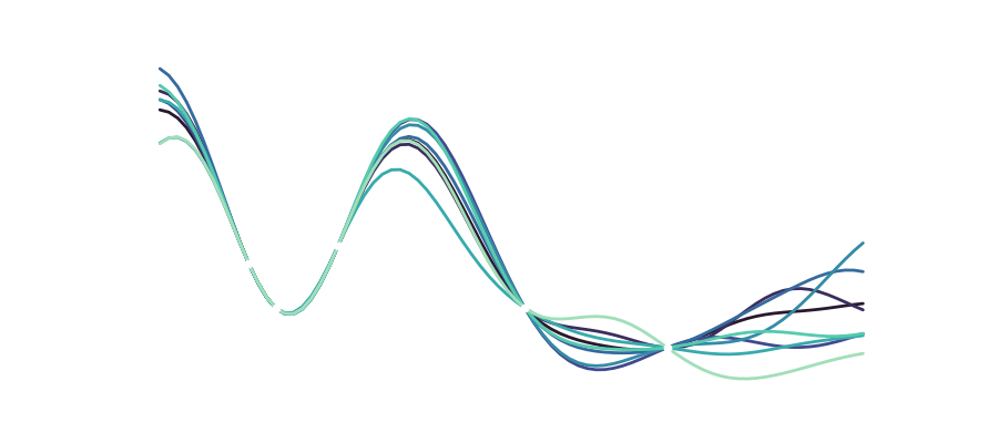
The second animation shows you all of the generated trajectories over the course of training, where early models are depicted in dark colors and late models in bright ones. Here it is quite cool to see that the first two models really didn’t yet train enough to capture the system’s dynamics and immediately leave the trajectory once the 15 context samples ran out. From there you can observe that models that have trained for longer better approximate the true state shown in blue. Now again after one loop or so the even the trained models diverge due to minor differences at some point in the past, but it is worth noting, that the trained recurrent networks (especially the ones with more training time) correctly characterize the dynamical system with its two lobes spanning the 3D space. Now what that means is that you can use the network to describe the system and you probably have a useful model when combined with some data fusion process like Kalman filtering.


Feel free to have a look at the full code and play around with the model yourself @github-gist.

How Natural Interaction can Bootstrap Self-Supervised Learning

This has been in the works for quite some time now. If you find the ideas teased in the video interested take a look at the accompanying paper [1], to be presented at this years ICLR.


[1] A. Aubret*, M. R. Ernst*, C. Teuliere, and J. Triesch, “Time to augment self-supervised visual representation learning” in International Conference on Learning Representations (ICLR) (2023).

* Equal contribution

Uncertainty Estimation with Gaussian Processes

Gaussian Procress Regression (GPR) is a powerful tool to do uncertainty estimation for all kinds of problems including state estimation in robotics or machine learning of geospatial data. It enables you to get an uncertainty estimation given new incoming data and is related to the concept of Kalman filtering that was briefly mentioned on this blog before. In this post I show the basic building blocks of this method and how to code a GPR yourself using Python.

Background

Formally, a Gaussian process is a stochastic process and can be understood as a distribution over functions. The premise of this approach is that the function values themselves are random variables. When modeling a function as a Gaussian process, one makes an assumption that any finite number of sampled points form a multivariate normal distribution.

Thus, f(x) \sim GP(\mu, k) means that for any finite batch of function values \mathbf{f} = f(\mathbf{X}), where \mathbf{f} = \left[ f(\mathbf{x_1}, ..., f(\mathbf{x_n}))\right] \sim \mathcal{N}(\mu, K) holds.

One might ask why this assumption is useful. The main benefit of using Gaussian distributions is that they are incredibly nice to work with. The Gaussian family is self-conjugate and has a number of nice properties such as being closed under marginalization and closed under conditioning. This makes it a natural choice for Bayesian machine learning, where you have to specify a prior belief  and then marginalize over parameters to obtain a posterior predictive distribution.

Also, the multivariate normal distribution is entirely characterized by a mean vector and a covariance matrix.

Inference

So how does one make predictions based on observed (training) data? It is basically based on this formulation:

(1)    \begin{equation*} \left[ {\begin{array}{c} f \\f^* \end{array} } \right] = \mathcal{N}\left( \mu, \left[ {\begin{array}{cc} K + \sigma^2 \mathbb{I}_n & K_* \\K_*^T & K_{**} \\ \end{array} } \right]  \right). \end{equation*}

The equation above reflects the previously mentioned assumption of normality, but here we also differentiate training and testing points (the latter is marked with an asterisk). There’s also an additional assumption that training labels are corrupted by Gaussian noise, which is the \sigma part at the top left in the kernel-matrix above.

Now, it is possible to compute the conditional distribution of the test data:

(2)    \begin{eqnarray*} Cov(f^*) = K_{**} - K_*^T(K+\sigma^2 \mathbb{I}_n)^{-1}K_* \\ \mu(f^*) = K_*^T(K+\sigma^2 \mathbb{I}_n)^{-1}f. \end{eqnarray*}

These equations give us a formal way of calculating the predictive mean and covariances at the test points conditioned on the training data.


GP Kernels

To actually use the equations above, one has to find a way to model the covariances and cross-covariances between all combinations of training and testing data. To do this we assume a certain kernel function for modeling the covariances. There are multiple possible kernels and choosing the right kernel function is critical for achieving good model fit, because they determine the shape of the resulting function. In this post I choose a squared exponential kernel: k_{SqE}(x_1,x_2):= \sigma^2 \cdot \exp(-\|x_1-x_2\|^2_2)/(2 \cdot l^2)) with l>0 the lengthscale and \sigma^2>0 the signal variance. But feel free to try out another kernels, like Brownian k_B(x_1,x_2) := min(x_1,x_2) for example.

Once the hyperparameters are optimized, the kernel matrix can be plugged into the predictive equations for the mean and covariance of the test data to obtain concrete results.

Regression

One of the key features of GP regression is that we are modeling a function where we only have a limited number of observations. Yet, we are interested in the values (and uncertainties) at unobserved locations. This can be useful for weather prediction, as rainfall and temperatures are only measured at specific locations or for sensor readings that only occur every so often. Once you found a suitable kernel function for modeling the similarities between such data points distributed in space or time and you optimized the kernel function parameters using a training set, you can make predictions on the test set using the predictive equations.

Do it yourself with Python

Recall that I chose a squared exponential kernel, which itself is defined by a mean value M and a variance \sigma. We can quickly visualize this kernel to see what these two parameters do to the kernel.


Here is the kernel for our Python implementation:


class SquaredExponentialKernel:
    def __init__(self, sigma_f=1, length=1):
        self.sigma_f = sigma_f
        self.length = length

    def __call__(self, argument_1, argument_2):
        return float(self.sigma_f * np.exp(-(np.linalg.norm(argument_1 - argument_2)**2) / (2 * self.length**2)))


Let us shortly recall the formula:
Given training points x_1,...,x_n\in \mathbb{R}^m with values y_1,...,y_n\in \mathbb{R}, y = (y_i)\in \mathbb{R}^n with noise in each point \mathcal{N}_{0,\sigma} and points x_{n+1},...,x_k\in \mathbb{R}^m for which we want to predict the output, adapting our probability distribution leads to:

\mathcal{N}(K_*^T(K+\sigma^2 \mathbb{I}_n)^{-1}f, K_{**}-K_*^T(K+\sigma^2 \mathbb{I}_n)^{-1}K_*), with

K= (k(x_i,x_j))_{i,j\leq n}

K_*= (k(x_i,x_j))_{n+1\leq i, j\leq n}

K_{**}= (k(x_i,x_j))_{n+1\leq i,j}


And here we go with our main GPR class and a little visualization function:


# Helper function to calculate the respective covariance matrices
def cov_matrix(x1, x2, cov_function):
    return np.array([[cov_function(a, b) for a in x1] for b in x2])


class GPR:
    def __init__(self, data_x, data_y,
                 covariance_function=SquaredExponentialKernel(),
                 white_noise_sigma=0.0):
        self.noise = white_noise_sigma
        self.data_x = data_x
        self.data_y = data_y
        self.covariance_function = covariance_function

        # Store the inverse of covariance matrix of input (+ machine epsilon on diagonal) since it is needed for every prediction
        self._inverse_of_covariance_matrix_of_input = np.linalg.inv(
            cov_matrix(data_x, data_x, covariance_function) +
            (3e-7 + self.noise) * np.identity(len(self.data_x)))

        self._memory = None

    # function to predict output at new input values. Store the mean and covariance matrix in memory.

    def predict(self, at_values: np.array) -> np.array:
        k_lower_left = cov_matrix(self.data_x, at_values,
                                  self.covariance_function)
        k_lower_right = cov_matrix(at_values, at_values,
                                   self.covariance_function)

        # Mean.
        mean_at_values = np.dot(
            k_lower_left,
            np.dot(self.data_y,
                   self._inverse_of_covariance_matrix_of_input.T).T).flatten()

        # Covariance.
        cov_at_values = k_lower_right - \
            np.dot(k_lower_left, np.dot(
                self._inverse_of_covariance_matrix_of_input, k_lower_left.T))

        # Adding value larger than machine epsilon to ensure positive semi definite
        cov_at_values = cov_at_values + 3e-7 * np.ones(
            np.shape(cov_at_values)[0])

        var_at_values = np.diag(cov_at_values)

        self._memory = {
            'mean': mean_at_values,
            'covariance_matrix': cov_at_values,
            'variance': var_at_values
        }
        return mean_at_values


def plot_GPR(data_x, data_y, model, x, ax, color_index=1):

    mean = model.predict(x)
    std = np.sqrt(model._memory['variance'])

    for i in range(1, 4):
        ax.fill_between(x, y1=mean + i * std, y2=mean - i * std,
                        color=sns.color_palette('bright')[color_index], alpha=.3,)
        # label=f"mean plus/minus {i}*standard deviation")

    ax.plot(x, mean, label='mean', color=sns.color_palette(
        'bright')[color_index], linewidth=2)
    ax.scatter(data_x, data_y, label='data-points',
               color=sns.color_palette('bright')[color_index], s=30, zorder=100)
    
    pass

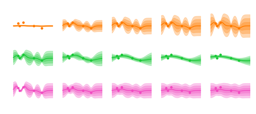
Now this is cool because now we can take a look at our GPR at work. The shaded areas represent 1,2,3 and 4 times the standard deviation. You can clearly see that uncertainty is low in the area where we have more data and it grows where we have no observations.


x_values = np.array([0, 0.3, 1, 3.1, 4.7])
y_values = np.array([1, 0, 1.4, 0, -0.9])
xlim = [-1, 7]
x = np.arange(xlim[0], xlim[1], 0.1)


fig, axes = plt.subplots(6, 1, figsize=(7, 9))
for i, ax in enumerate(axes.flatten()):
    x_val = x_values[:i]
    y_val = y_values[:i]
    model = GPR(x_val, y_val)
    plot_GPR(data_x=x_val, data_y=y_val, x=x,
             model=model, ax=ax, color_index=i)
    ax.set_xlim(xlim)
    ax.set_ylim([-6, 6])
plt.tight_layout()
plt.show()


Of course, we can also look at the different functions drawn from the distribution that make up our variance:

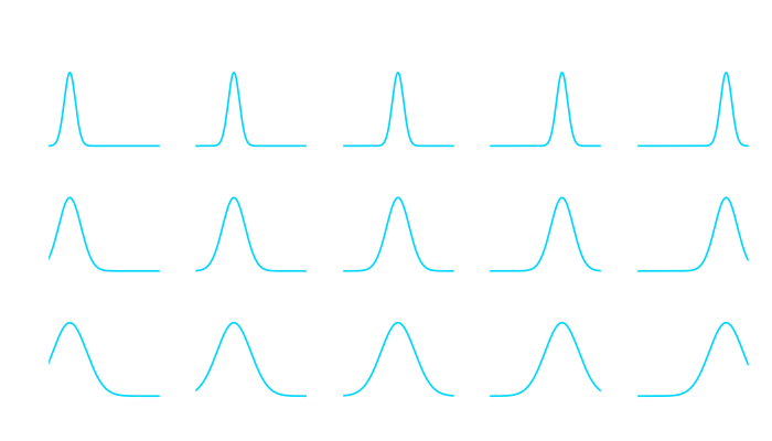
Another interesting aspect is that we of course still have the hyperparameters \sigma,l and the noise that can influence how we model our data. Varying these parameters looks like this:

Sigma mainly influences the uncertainty envelope, allowing for functions that more or less deviate from the mean. The length scale influences how smooth the curve becomes, and how curvy and bendy the functions get. And depending on the amount of noise we assume in the data the predicted functions are more or less tied to the observation points.

Conclusion

A GP model is a non-parametric model which is flexible and can fit many kinds of data, including geospatial and time series data. At the core of GP regression is the specification of a suitable kernel function, or measure of similarity between data points. The tractability of the Gaussian distribution means that one can find closed-form expressions for the posterior predictive distribution conditioned on training data. For a deep dive, feel free to look at the book Gaussian Processes for Machine Learning by Rasmussen and Williams.

Using Blender for 3D Animation and Modelling

The first long-term support of the 3.x series is here!
Discover Blender 3.3 LTS

So this is great news. Blender has been a staple of Open Source software for as long as I can remember and you can basically do everything with it. It has a steep learning curve, so you need to put in some time and effort but it really is an amazing piece of software. See their blog-post on how Blender was used to create the effects of the recent Bollywood blockbuster “RRR”.

A gatekeeper for me was always GPU acceleration. I never really had a personal computer that is that powerful or in recent time even has had a dedicated GPU, but with Blender 3 they offer GPU acceleration using Apple’s Metal framework and this is a Gamechanger even if you are just on a M1 Macbook Air, as a I am.

So to dive right in I chose the now famous Blender donut tutorial series to practice my skills and oh boy this is fun. With all the scripting support it also is an incredible tool to do datavisualization and I can’t wait to spend more time with it.

As for donuts, I just find it amazing that I basically created this out of thin air. Here’s my take: