This has been in the works for quite some time now. If you find the ideas teased in the video interested take a look at the accompanying paper [1], to be presented at this years ICLR.
* Equal contribution
I am a coffee-enthusiast and AI researcher
This has been in the works for quite some time now. If you find the ideas teased in the video interested take a look at the accompanying paper [1], to be presented at this years ICLR.
* Equal contribution
Gaussian Procress Regression (GPR) is a powerful tool to do uncertainty estimation for all kinds of problems including state estimation in robotics or machine learning of geospatial data. It enables you to get an uncertainty estimation given new incoming data and is related to the concept of Kalman filtering that was briefly mentioned on this blog before. In this post I show the basic building blocks of this method and how to code a GPR yourself using Python.
Formally, a Gaussian process is a stochastic process and can be understood as a distribution over functions. The premise of this approach is that the function values themselves are random variables. When modeling a function as a Gaussian process, one makes an assumption that any finite number of sampled points form a multivariate normal distribution.
Thus, means that for any finite batch of function values
, where
holds.
One might ask why this assumption is useful. The main benefit of using Gaussian distributions is that they are incredibly nice to work with. The Gaussian family is self-conjugate and has a number of nice properties such as being closed under marginalization and closed under conditioning. This makes it a natural choice for Bayesian machine learning, where you have to specify a prior belief and then marginalize over parameters to obtain a posterior predictive distribution.
Also, the multivariate normal distribution is entirely characterized by a mean vector and a covariance matrix.
So how does one make predictions based on observed (training) data? It is basically based on this formulation:
(1)
The equation above reflects the previously mentioned assumption of normality, but here we also differentiate training and testing points (the latter is marked with an asterisk). There’s also an additional assumption that training labels are corrupted by Gaussian noise, which is the part at the top left in the kernel-matrix above.
Now, it is possible to compute the conditional distribution of the test data:
(2)
These equations give us a formal way of calculating the predictive mean and covariances at the test points conditioned on the training data.
To actually use the equations above, one has to find a way to model the covariances and cross-covariances between all combinations of training and testing data. To do this we assume a certain kernel function for modeling the covariances. There are multiple possible kernels and choosing the right kernel function is critical for achieving good model fit, because they determine the shape of the resulting function. In this post I choose a squared exponential kernel: with
the lengthscale and
the signal variance. But feel free to try out another kernels, like Brownian
for example.
Once the hyperparameters are optimized, the kernel matrix can be plugged into the predictive equations for the mean and covariance of the test data to obtain concrete results.
One of the key features of GP regression is that we are modeling a function where we only have a limited number of observations. Yet, we are interested in the values (and uncertainties) at unobserved locations. This can be useful for weather prediction, as rainfall and temperatures are only measured at specific locations or for sensor readings that only occur every so often. Once you found a suitable kernel function for modeling the similarities between such data points distributed in space or time and you optimized the kernel function parameters using a training set, you can make predictions on the test set using the predictive equations.
Recall that I chose a squared exponential kernel, which itself is defined by a mean value and a variance
. We can quickly visualize this kernel to see what these two parameters do to the kernel.

Here is the kernel for our Python implementation:
class SquaredExponentialKernel:
    def __init__(self, sigma_f=1, length=1):
        self.sigma_f = sigma_f
        self.length = length

    def __call__(self, argument_1, argument_2):
        return float(self.sigma_f * np.exp(-(np.linalg.norm(argument_1 - argument_2)**2) / (2 * self.length**2)))
Let us shortly recall the formula:
Given training points with values
,
with noise in each point
and points
for which we want to predict the output, adapting our probability distribution leads to:
, with
And here we go with our main GPR class and a little visualization function:
# Helper function to calculate the respective covariance matrices
def cov_matrix(x1, x2, cov_function):
    return np.array([[cov_function(a, b) for a in x1] for b in x2])


class GPR:
    def __init__(self, data_x, data_y,
                 covariance_function=SquaredExponentialKernel(),
                 white_noise_sigma=0.0):
        self.noise = white_noise_sigma
        self.data_x = data_x
        self.data_y = data_y
        self.covariance_function = covariance_function

        # Store the inverse of covariance matrix of input (+ machine epsilon on diagonal) since it is needed for every prediction
        self._inverse_of_covariance_matrix_of_input = np.linalg.inv(
            cov_matrix(data_x, data_x, covariance_function) +
            (3e-7 + self.noise) * np.identity(len(self.data_x)))

        self._memory = None

    # function to predict output at new input values. Store the mean and covariance matrix in memory.

    def predict(self, at_values: np.array) -> np.array:
        k_lower_left = cov_matrix(self.data_x, at_values,
                                  self.covariance_function)
        k_lower_right = cov_matrix(at_values, at_values,
                                   self.covariance_function)

        # Mean.
        mean_at_values = np.dot(
            k_lower_left,
            np.dot(self.data_y,
                   self._inverse_of_covariance_matrix_of_input.T).T).flatten()

        # Covariance.
        cov_at_values = k_lower_right - \
            np.dot(k_lower_left, np.dot(
                self._inverse_of_covariance_matrix_of_input, k_lower_left.T))

        # Adding value larger than machine epsilon to ensure positive semi definite
        cov_at_values = cov_at_values + 3e-7 * np.ones(
            np.shape(cov_at_values)[0])

        var_at_values = np.diag(cov_at_values)

        self._memory = {
            'mean': mean_at_values,
            'covariance_matrix': cov_at_values,
            'variance': var_at_values
        }
        return mean_at_values


def plot_GPR(data_x, data_y, model, x, ax, color_index=1):

    mean = model.predict(x)
    std = np.sqrt(model._memory['variance'])

    for i in range(1, 4):
        ax.fill_between(x, y1=mean + i * std, y2=mean - i * std,
                        color=sns.color_palette('bright')[color_index], alpha=.3,)
        # label=f"mean plus/minus {i}*standard deviation")

    ax.plot(x, mean, label='mean', color=sns.color_palette(
        'bright')[color_index], linewidth=2)
    ax.scatter(data_x, data_y, label='data-points',
               color=sns.color_palette('bright')[color_index], s=30, zorder=100)

    pass
Now this is cool because now we can take a look at our GPR at work. The shaded areas represent 1,2,3 and 4 times the standard deviation. You can clearly see that uncertainty is low in the area where we have more data and it grows where we have no observations.

x_values = np.array([0, 0.3, 1, 3.1, 4.7])
y_values = np.array([1, 0, 1.4, 0, -0.9])
xlim = [-1, 7]
x = np.arange(xlim[0], xlim[1], 0.1)


fig, axes = plt.subplots(6, 1, figsize=(7, 9))
for i, ax in enumerate(axes.flatten()):
    x_val = x_values[:i]
    y_val = y_values[:i]
    model = GPR(x_val, y_val)
    plot_GPR(data_x=x_val, data_y=y_val, x=x,
             model=model, ax=ax, color_index=i)
    ax.set_xlim(xlim)
    ax.set_ylim([-6, 6])
plt.tight_layout()
plt.show()
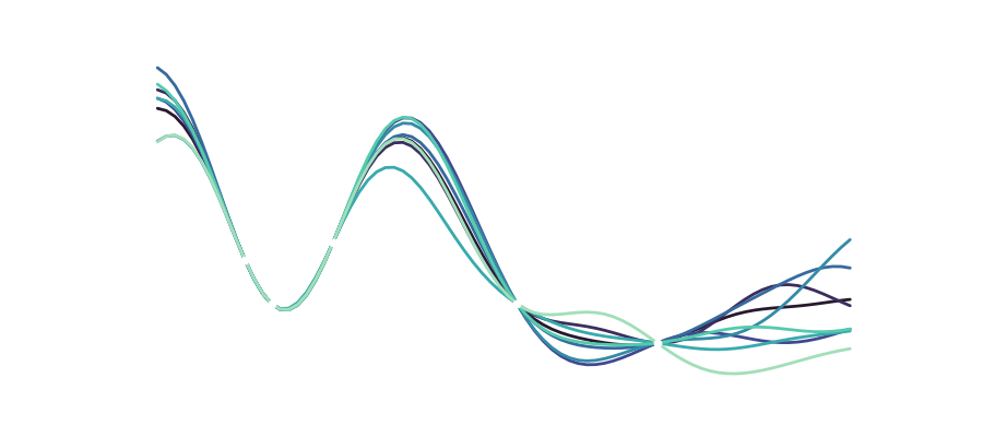
Of course, we can also look at the different functions drawn from the distribution that make up our variance:

Another interesting aspect is that we of course still have the hyperparameters ,
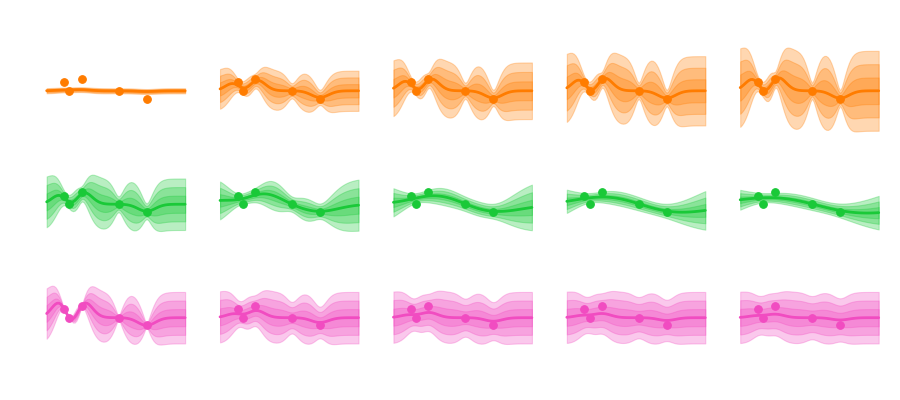
and the noise that can influence how we model our data. Varying these parameters looks like this:

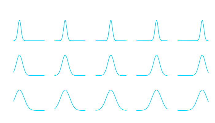
Sigma mainly influences the uncertainty envelope, allowing for functions that more or less deviate from the mean. The length scale influences how smooth the curve becomes, and how curvy and bendy the functions get. And depending on the amount of noise we assume in the data the predicted functions are more or less tied to the observation points.
A GP model is a non-parametric model which is flexible and can fit many kinds of data, including geospatial and time series data. At the core of GP regression is the specification of a suitable kernel function, or measure of similarity between data points. The tractability of the Gaussian distribution means that one can find closed-form expressions for the posterior predictive distribution conditioned on training data. For a deep dive, feel free to look at the book Gaussian Processes for Machine Learning by Rasmussen and Williams.
The first long-term support of the 3.x series is here!
Discover Blender 3.3 LTS
So this is great news. Blender has been a staple of Open Source software for as long as I can remember and you can basically do everything with it. It has a steep learning curve, so you need to put in some time and effort but it really is an amazing piece of software. See their blog-post on how Blender was used to create the effects of the recent Bollywood blockbuster “RRR”.
A gatekeeper for me was always GPU acceleration. I never really had a personal computer that is that powerful or in recent time even has had a dedicated GPU, but with Blender 3 they offer GPU acceleration using Apple’s Metal framework and this is a Gamechanger even if you are just on a M1 Macbook Air, as a I am.
So to dive right in I chose the now famous Blender donut tutorial series to practice my skills and oh boy this is fun. With all the scripting support it also is an incredible tool to do datavisualization and I can’t wait to spend more time with it.
As for donuts, I just find it amazing that I basically created this out of thin air. Here’s my take:
In collaboration with the Metal engineering team at Apple, we are excited to announce support for GPU-accelerated PyTorch training on Mac.
It’s about time. It has been 18 months since the first M1 chips shipped and finally we got some support for the advanced GPUs on these chips. Being able to leverage your own local machine for simple Pytorch tasks and even just doing local testing of bigger projects is of tremendous value. One thing I am still confused about is that all of this technology still just uses the ‘standard’ GPU cores and there is still no way to access the custom Neural Engine of the chip. This would make inference on device even better. But it’s up to Apple to give access to their internal APIs.
I spent the last few months working as a research assistant in artificial intelligence at the Frankfurt Institute for Advanced Studies. With the global COVID-19 situation almost all parts of the scientific workflow went digital. I was working from home, logging into the office computers and high performance clusters via SSH, but all in all this was not that much different than programming and logging on from the office. One thing that has changed significantly, though, is conferences.
As large gatherings of people are potential COVID hotspots it totally makes sense for conferences to go virtual, … at least for this year. And there is tremendous potential in having virtual events: Talks get recorded more frequently, allowing for a more flexible schedule; pre-recorded talks make sure that everyone keeps within their time-slot; it’s more inclusive for people who otherwise cannot afford to attend and last but definitely not least it’s better for global climate for not having people fly all over the world.
I firmly believe that the academic world should learn from this special situation and incorporate some of the up-sides of having virtual events into future conferences: Maybe an alternating schedule (virtual/in-person) would be a good idea. But right now I feel everything is going to go back to as it was before.
Why do I think this…? Well, I think people enjoy being with each other and we have not figured out how to do the networking part conferences yet. For me it becomes most apparent with poster-sessions. Sure you cannot drink a beer at bar with your colleagues when you are stuck behind your webcam at your desk, but that was never going to be. The poster-session format is partly social interaction with a presenter and it fails badly at virtual conferences, and actually there is no real reason why.
So there might be conferences that actually do what I suggest next, so I apologize beforehand, but the three conferences I attended this year either scrubbed the poster session and made posters downloadable or made them short 5 min prerecorded talks. I understand the notion that this is the easiest way but I am kind of disappointed that we have not figured out something better.
In my opinion there’s actually two sides to the problem: conceptualization and software.
You have to think about what makes a poster-session a poster-session. How does it work and why does it work? Inspire from the real world and take it to the virtual one.
Start with a showcase. There needs to be a website where you can visually scroll through all of the posters. This is a no-brainer: don’t just go with abstracts and links and no, it doesn’t have to be a fancy 3D virtual floor. Just make it a long scrollable website with BIG images. People have spent time designing these posters, this is what catches our attention at the poster session. Have little hearts or thumbs-up icons next to the images to indicate whether some poster creates enthusiasm among the participants.
When you click on a poster you should be pulled into a virtual conference room, like a zoom call, where the presenter talks about her poster and answers questions. Now here comes the software part: Simple screen sharing is not enough, we need a simplified powerpoint for posters/documents. Conceptually it should be like prezi, because the poster is the whole canvas, but there should be simple tools that analyze the PDF and make it easy to highlight regions like boxes and round-rects and of course you should be able to pan and zoom around. Moreover it should not be a video-stream! Something like this needs to be rendered client-side. These posters are smaller than your average hd video and they are vector-based, making them effectively resolution independent. With client-side rendering the participants can decide for themselves on which parts of the canvas they would like to focus.
To end this little blogpost I want to showcase what I came up with for this year’s ESANN conference. Let me be clear, this was way more work than a simple poster. But given the right software it should be feasable to transform any PDF into something where you can zoom around and highlight passages in a similar manner [1].
On a little side-note I’m still on the lookout for a cool PhD position, so please get in touch if you want to work with me!
[1] If you liked that video, you can of course take a look at the corresponding paper:
Ernst M.R., Triesch J., Burwick T. (2020). Recurrent Feedback Improves Recognition of Partially Occluded Objects. In Proceedings of the 28th European Symposium on Artificial Neural Networks, Computational Intelligence and Machine Learning (ESANN)